Physics validation

MHX validation tests have explicit physics gates, not just smoke-run assertions. The suite starts from exact resistive diffusion of a single Fourier mode and now includes Harris tearing eigenvalue checks, nonlinear energy-budget identities, duration guards, Orszag–Tang morphology, decaying turbulence, forced turbulent-reconnection media with a validation-only readiness gate, double-Harris promotion/convergence evidence, seed-QI, neural-ODE reproducibility, and restartable campaign-executor artifacts.

Exact resistive decay

With zero flow and one flux mode,

\[ \psi(x,y,0)=\cos(k_x x + k_y y), \qquad \omega(x,y,0)=0, \]

the reduced-MHD flux equation collapses to

\[ \partial_t\psi = \eta\nabla^2\psi. \]

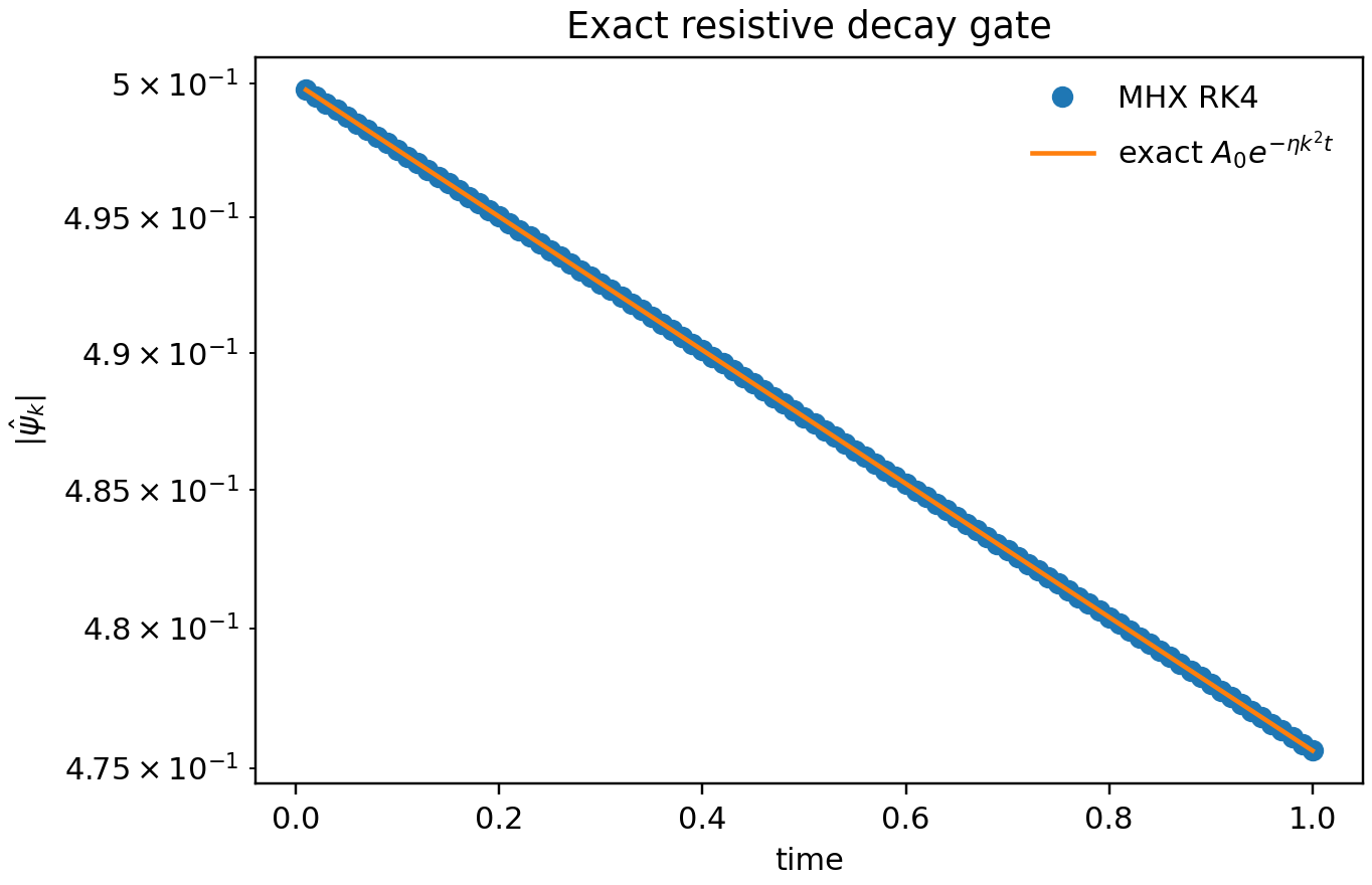
The exact solution is

\[ \psi(x,y,t)=\psi(x,y,0)\exp(-\eta |k|^2 t), \qquad |k|^2=k_x^2+k_y^2, \]

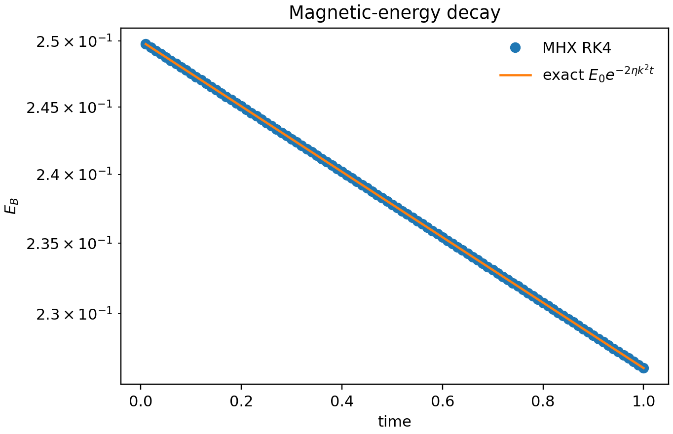
and magnetic energy must decay as

\[ E_B(t)=E_B(0)\exp(-2\eta |k|^2t). \]

These gates test the spectral Laplacian sign convention, RK4 time stepping, mode diagnostics, energy diagnostics, output files, and plotting path.

Run the validation:

mhx benchmark decay --outdir outputs/benchmarks/resistive_decay

Expected files:

• outputs/benchmarks/resistive_decay/diagnostics.json

• outputs/benchmarks/resistive_decay/validation.json

• outputs/benchmarks/resistive_decay/decay_history.npz

• outputs/benchmarks/resistive_decay/figures/decay_amplitude.png

• outputs/benchmarks/resistive_decay/figures/decay_energy.png

• outputs/benchmarks/resistive_decay/figures/decay_relative_error.png

Regenerate the documentation figures:

python examples/make_validation_media.py

Run every active FAST validation gate and write a single reviewer-facing summary:

mhx validate all --outdir outputs/validation_suite

The suite writes validation_suite.json, validation_suite.md, artifact_manifest.json, and one subdirectory per validation case.

Nonlinear Orszag–Tang reduced-MHD gate

MHX includes a solver-generated nonlinear Orszag–Tang validation case:

mhx benchmark orszag-tang --outdir outputs/benchmarks/orszag_tang_vortex --movies

The initial condition adapts the classic Orszag–Tang two-dimensional MHD vortex to the incompressible reduced-MHD variables:

\[ \phi=\cos x+\cos y,\qquad \psi=\cos y+\frac{1}{2}\cos 2x, \]

giving

\[ \mathbf{v}_\perp=(-\sin y,\sin x),\qquad \mathbf{B}_\perp=(-\sin y,\sin 2x). \]

The validation checks finite fields, monotone resistive-viscous energy decay, net dissipation, high-wavenumber growth in current density and vorticity, and spectral preservation of \(\nabla\cdot\mathbf{B}_\perp=0\). This is not a compressible full-MHD shock benchmark; it is the nonlinear reduced-MHD example used by the README media and extension tutorials.

Expected files:

• outputs/benchmarks/orszag_tang_vortex/diagnostics.json

• outputs/benchmarks/orszag_tang_vortex/validation.json

• outputs/benchmarks/orszag_tang_vortex/orszag_tang_vortex.npz

• outputs/benchmarks/orszag_tang_vortex/figures/orszag_tang_summary.png

• outputs/benchmarks/orszag_tang_vortex/figures/orszag_tang_current.gif

• outputs/benchmarks/orszag_tang_vortex/figures/orszag_tang_vorticity.gif

Decaying turbulence and forced turbulent reconnection

The turbulence validations exercise nonlinear advection, current-sheet formation, and reconnection-proxy diagnostics without claiming converged turbulent reconnection rates. The reduced-MHD equations remain

\[ \partial_t\psi + [\phi,\psi] = \eta\nabla^2\psi, \qquad \partial_t\omega + [\phi,\omega] = [\psi,\nabla^2\psi] + \nu\nabla^2\omega + F_\omega , \]

where the decaying case sets \(F_\omega=0\) and the forced current-sheet case uses a weak deterministic large-scale vorticity forcing. The decaying gate checks finite arrays, total-energy decay, current amplification, and high-\(k\) transfer. The forced gate checks finite arrays, bounded injected energy, current amplification, and a reconnection proxy built from X/O critical-point flux separation when available, with a documented max-min flux fallback.

Run the validations:

mhx benchmark decaying-turbulence --outdir outputs/benchmarks/decaying_mhd_turbulence --movies
mhx benchmark forced-turbulent-reconnection --outdir outputs/benchmarks/forced_turbulent_reconnection --movies
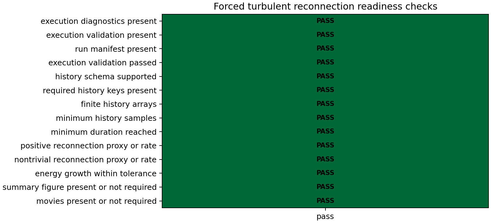
mhx benchmark forced-turbulent-reconnection-readiness-check outputs/benchmarks/forced_turbulent_reconnection

Expected files:

• outputs/benchmarks/decaying_mhd_turbulence/decaying_mhd_turbulence.npz

• outputs/benchmarks/decaying_mhd_turbulence/figures/decaying_mhd_turbulence_summary.png

• outputs/benchmarks/forced_turbulent_reconnection/forced_turbulent_reconnection.npz

• outputs/benchmarks/forced_turbulent_reconnection/figures/forced_turbulent_reconnection_summary.png

• outputs/benchmarks/forced_turbulent_reconnection/readiness/promotion_readiness.json

• outputs/benchmarks/forced_turbulent_reconnection/readiness/figures/promotion_matrix.png

• optional flux/current GIFs under each figures/ directory

The readiness matrix is a validation-only claim boundary for the forced current-sheet replay. It requires finite histories, enough saved samples, minimum duration, nontrivial reconnecting-flux or reconnection-rate proxy, bounded total-energy growth, and the expected summary/movie artifacts.

These examples are literature-anchored to 2-D MHD turbulence and turbulent-reconnection studies, including the current-sheet/turbulence diagnostic tradition used by Servidio and collaborators and the broader Lazarian–Vishniac picture of turbulence-assisted reconnection. The current MHX examples are pedagogical 2-D reduced-MHD validation artifacts, not 3-D fast-reconnection production evidence.

Source links:

• Turbulence implementation

• Critical-point diagnostics

• Turbulence tests

Validation figures

The numerical mode amplitude is visually indistinguishable from \(A_0\exp(-\eta |k|^2t)\) at FAST settings.

The magnetic energy follows the required \(E_B(0)\exp(-2\eta |k|^2t)\) law.

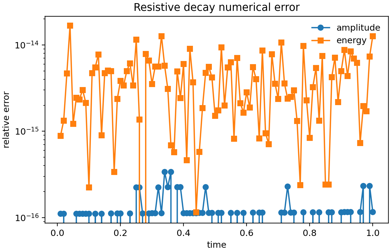
The relative-error plot is the reviewer-facing numerical gate. The corresponding unit test fails if amplitude, energy, fitted rate, monotonicity, or final-field L2 gates exceed documented tolerances.

Literature anchors

The exact-decay test is deliberately simpler than a tearing eigenvalue problem, but it validates the finite-resistivity induction term used in classical resistive-MHD reconnection theory. The benchmark roadmap then builds toward the FKR tearing mode, plasmoid instability scalings, and ideal-tearing regimes. For broader reconnection context, see Biskamp’s Magnetic Reconnection in Plasmas and the MHX literature page.

Source links

• Validation implementation

• Validation tests

• Plotting helpers

Seed-robust QI validation

MHX now includes a FAST seed-robust quality-indicator lane. It adds tiny smooth, zero-mean perturbations to the reduced-MHD tearing initial condition and gates whether gamma_fit, final energies, and spectral magnetic-divergence diagnostics are stable across the seed ensemble.

The CLI command is:

mhx benchmark seed-robust-qi --outdir outputs/benchmarks/seed_robust_qi

The manifest is claim_level = "validation". This supports only local FAST metric-sensitivity claims, not turbulent ensemble uncertainty quantification or production plasmoid statistics.

Source anchors:

• QI implementation

• Validation-suite registry

• QI documentation

Reconnection scaling gates

The next validation layer checks that MHX’s analytic benchmark scaffolds encode the literature exponents that future numerical benchmarks must recover.

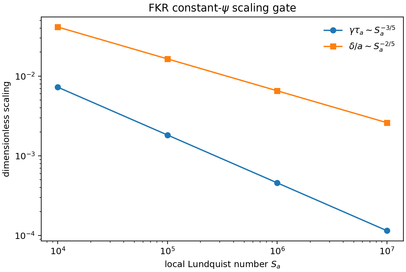
For constant-\(\psi\) FKR tearing, using the Harris-sheet proxy

\[ \Delta'a = 2\left[(ka)^{-1}-ka\right], \]

MHX gates the order-unity-coefficient-free scalings

\[ \gamma\tau_a \sim S_a^{-3/5}(ka)^{2/5}(\Delta'a)^{4/5}, \qquad \delta/a \sim S_a^{-2/5}(ka)^{-2/5}(\Delta'a)^{1/5}. \]

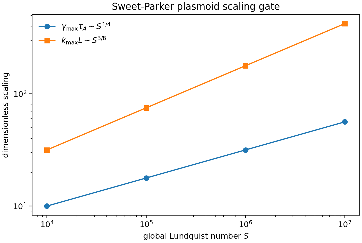
For a Sweet-Parker current sheet, the Loureiro–Schekochihin–Cowley plasmoid theory predicts

\[ \gamma_{\max}\tau_A \sim S^{1/4}, \qquad k_{\max}L \sim S^{3/8}. \]

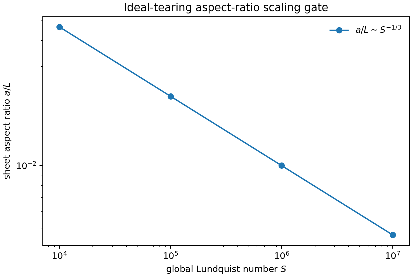
For ideal tearing, MHX checks the Pucci–Velli aspect-ratio scaling

\[ a/L \sim S^{-1/3}. \]

Run the scaling gates:

mhx benchmark scaling --outdir outputs/benchmarks/reconnection_scaling

Expected files:

• outputs/benchmarks/reconnection_scaling/diagnostics.json

• outputs/benchmarks/reconnection_scaling/validation.json

• outputs/benchmarks/reconnection_scaling/scaling_history.npz

• outputs/benchmarks/reconnection_scaling/figures/fkr_scaling.png

• outputs/benchmarks/reconnection_scaling/figures/plasmoid_scaling.png

• outputs/benchmarks/reconnection_scaling/figures/ideal_tearing_scaling.png

These gates do not prove the PDE solver has recovered FKR or plasmoid growth. They make the expected exponents explicit, tested, plotted, and reviewable so that future eigenmode and nonlinear-current-sheet benchmarks have fixed targets.

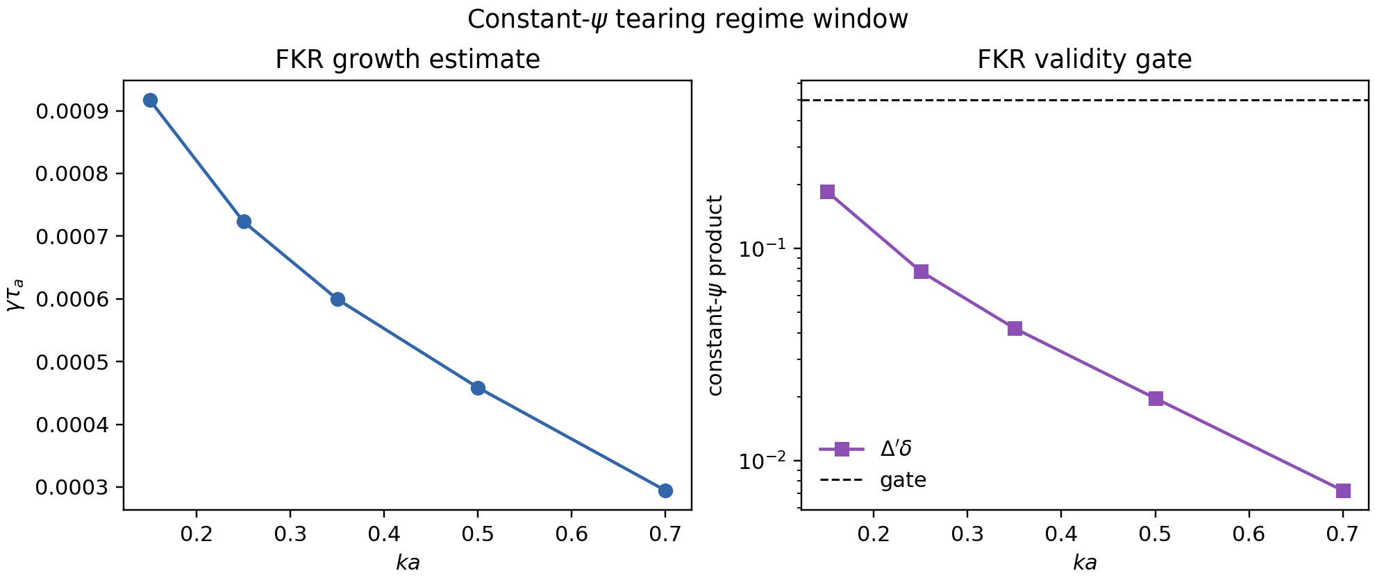
FKR constant-psi regime window

The FKR estimate is only appropriate in a restricted asymptotic window. MHX now ships a separate analytic gate that samples wavenumbers at fixed local Lundquist number and checks:

\[ \Delta'a > 0,\qquad \delta/a \le \delta_{\max},\qquad \Delta'\delta \le \epsilon_{\max}. \]

The last condition is the constant-\(\psi\) gate; large values move toward the Coppi large-\(\Delta'\) regime and should not be judged against the FKR constant-\(\psi\) scaling.

mhx benchmark fkr-window --outdir outputs/benchmarks/fkr_window

Expected files:

• outputs/benchmarks/fkr_window/diagnostics.json

• outputs/benchmarks/fkr_window/validation.json

• outputs/benchmarks/fkr_window/fkr_window.npz

• outputs/benchmarks/fkr_window/figures/fkr_constant_psi_window.png

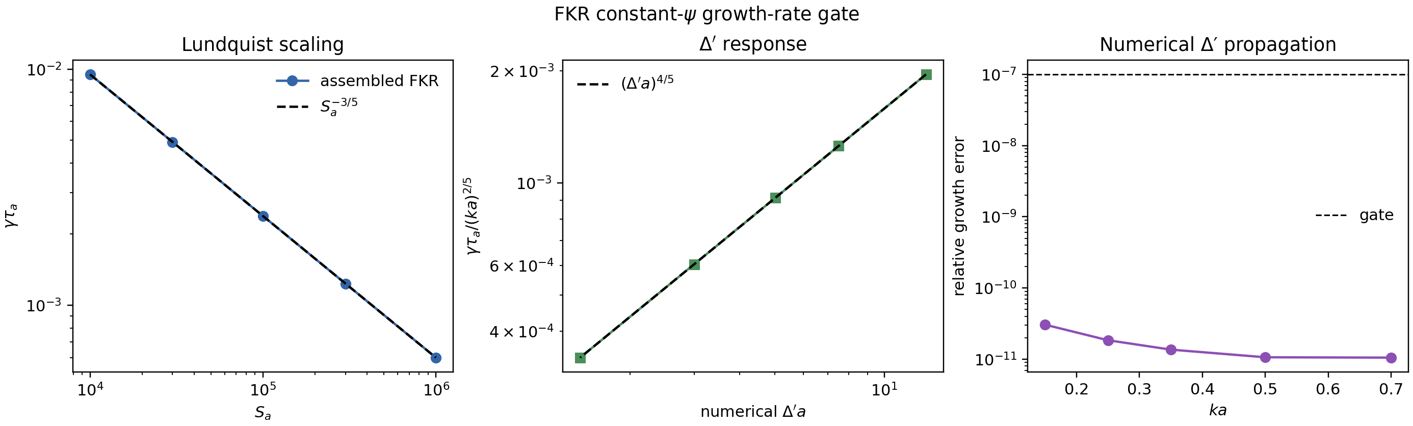
FKR growth-rate gate

The next layer converts the numerically recovered Harris outer-region \(\Delta'a\) into the FKR constant-\(\psi\) growth-rate estimate. MHX gates

\[ \gamma\tau_a \propto S_a^{-3/5} \]

at fixed \(ka\) and

\[ \frac{\gamma\tau_a}{(ka)^{2/5}} \propto (\Delta'a)^{4/5} \]

at fixed \(S_a\). The \(\Delta'a\) values used in the second scan come from the same backward-integration outer solve used by the Harris Delta-prime gate, so the benchmark now checks propagation from numerical outer matching into the growth-rate assembly.

mhx benchmark fkr-growth --outdir outputs/benchmarks/fkr_growth_rate

Expected files:

• outputs/benchmarks/fkr_growth_rate/diagnostics.json

• outputs/benchmarks/fkr_growth_rate/validation.json

• outputs/benchmarks/fkr_growth_rate/fkr_growth_rate.npz

• outputs/benchmarks/fkr_growth_rate/figures/fkr_growth_rate.png

This is still an asymptotic growth-rate assembly gate, not a full resistive inner-layer or global eigenvalue solve. The direct eigenvalue gate below closes one targeted part of that gap for a published Harris-sheet test case; broader FKR/Coppi scans still require a documented asymptotic-resolution study.

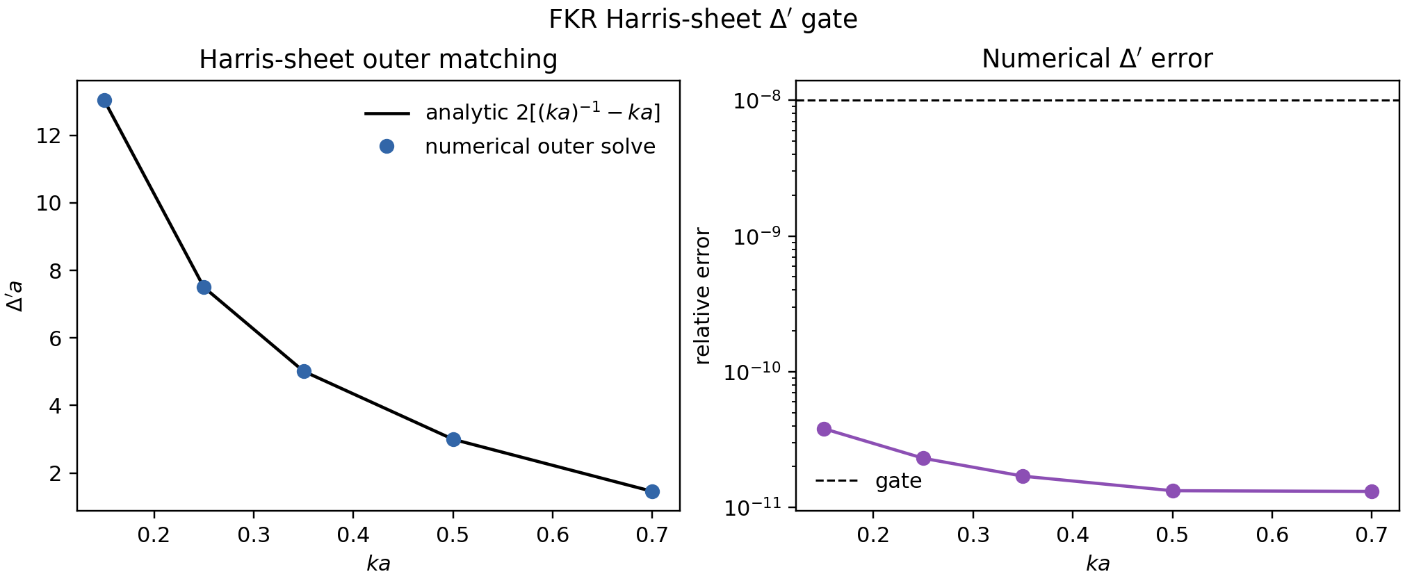
Harris-sheet Delta-prime gate

The first numerical tearing-specific validation is the Harris-sheet ideal outer equation. With

\[ B_y/B_0=\tanh(x/a),\qquad \xi=x/a, \]

the zero-inertia outer equation for the tearing-parity flux eigenfunction is

\[ \frac{d^2\psi}{d\xi^2} - \left[(ka)^2 - 2\,\operatorname{sech}^2\xi\right]\psi=0. \]

The decaying solution on each side of the sheet gives the FKR matching parameter

\[ \Delta'a = 2\frac{\psi'(0^+)}{\psi(0)} =2\left[(ka)^{-1}-ka\right]. \]

MHX now integrates this outer ODE numerically from large positive \(\xi\) back to the resonant surface and gates the recovered \(\Delta'a\) against the analytic formula. This is more substantial than plotting the formula, but it still is not the full resistive inner-layer eigenvalue solve.

mhx benchmark harris-delta-prime --outdir outputs/benchmarks/harris_delta_prime

Expected files:

• outputs/benchmarks/harris_delta_prime/diagnostics.json

• outputs/benchmarks/harris_delta_prime/validation.json

• outputs/benchmarks/harris_delta_prime/harris_delta_prime.npz

• outputs/benchmarks/harris_delta_prime/figures/harris_delta_prime.png

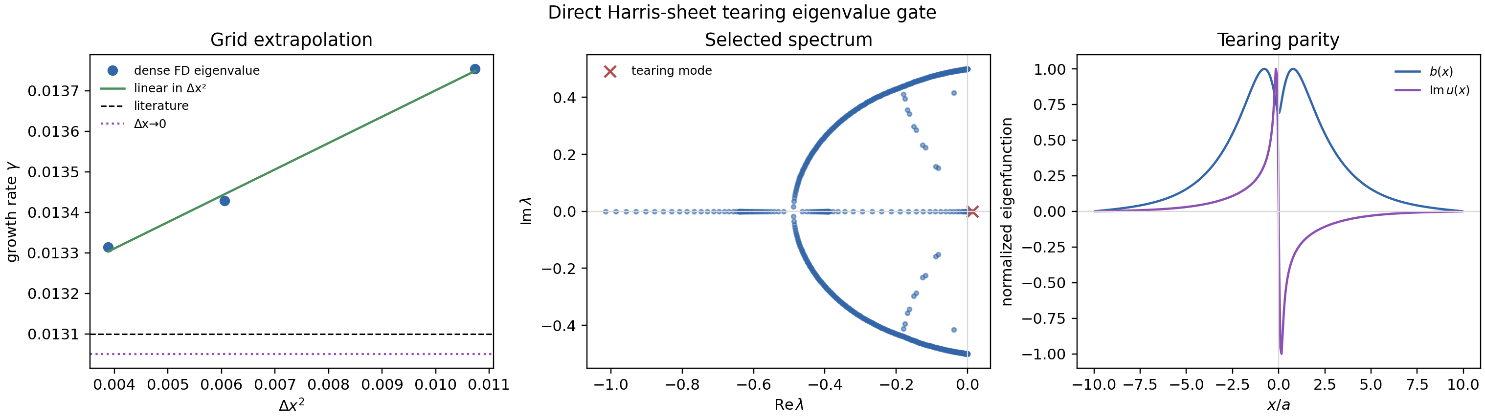
Direct Harris-sheet tearing eigenvalue gate

MHX now includes a direct 1D linear tearing eigenproblem benchmark anchored to published reduced-MHD calculations. For a Harris sheet,

\[ B_y/B_0=\tanh(x/a), \]

normal-mode perturbations proportional to \(\exp(iky+\sigma t)\) satisfy the inviscid linear reduced-MHD system

\[ \sigma\left(\frac{d^2}{dx^2}-k^2\right)u = ikB\left(\frac{d^2}{dx^2}-k^2\right)b -ikB''b, \]

\[ \sigma b = ikBu +S^{-1}\left(\frac{d^2}{dx^2}-k^2\right)b. \]

The benchmark uses conducting/no-slip perturbation boundaries,

\[ u=b=0\qquad \text{at}\qquad x=\pm d, \]

with \(S=1000\), \(ka=0.5\), and \(d/a=10\). It solves the dense finite-difference operator on three grids, extrapolates the growth rate linearly in \(\Delta x^2\), and gates against the published tearing eigenvalue \(\gamma\simeq0.0131\). Additional gates check that the selected eigenvalue is real and positive, the dense eigenpair residual is small, grid refinement decreases the finite-grid growth rate, and the selected mode has tearing parity: \(b(x)=b(-x)\) with odd stream-function perturbation. A stable-control solve at \(ka=1.2\) checks the same operator has no positive-growth eigenvalue outside the tearing-unstable \(0<ka<1\) interval.

Run the gate:

mhx benchmark linear-tearing-eigenvalue \
  --outdir outputs/benchmarks/linear_tearing_eigenvalue

Expected files:

• outputs/benchmarks/linear_tearing_eigenvalue/diagnostics.json

• outputs/benchmarks/linear_tearing_eigenvalue/validation.json

• outputs/benchmarks/linear_tearing_eigenvalue/linear_tearing_eigenvalue.npz

• outputs/benchmarks/linear_tearing_eigenvalue/figures/linear_tearing_eigenvalue.png

This is a materially stronger tearing validation than the analytic scaling and outer-region gates, but it is still a single reference eigenproblem. It does not yet establish production nonlinear reconnection fidelity, Coppi-regime dispersion curves, or plasmoid dynamics.

Finite-domain tearing dispersion gate

The next validation layer repeats the same finite-difference eigenproblem over a small \(ka\) scan. This is deliberately a FAST finite-domain gate, not a production asymptotic scan. It checks:

\[ \operatorname{Re}\lambda(ka)>0 \quad\text{for sampled}\quad 0<ka<1, \]

\[ \operatorname{Re}\lambda(ka)\le 0 \quad\text{for sampled}\quad ka>1, \]

plus dense eigenpair residuals and the same \(ka=0.5\) literature anchor used by the direct eigenvalue gate. The default samples are \(ka=(0.3,0.5,0.7,0.9,1.1,1.2)\) at \(S=1000\) and \(d/a=10\).

Run the scan:

mhx benchmark linear-tearing-dispersion \
  --outdir outputs/benchmarks/linear_tearing_dispersion

Expected files:

• outputs/benchmarks/linear_tearing_dispersion/diagnostics.json

• outputs/benchmarks/linear_tearing_dispersion/validation.json

• outputs/benchmarks/linear_tearing_dispersion/linear_tearing_dispersion.npz

• outputs/benchmarks/linear_tearing_dispersion/figures/linear_tearing_dispersion.png

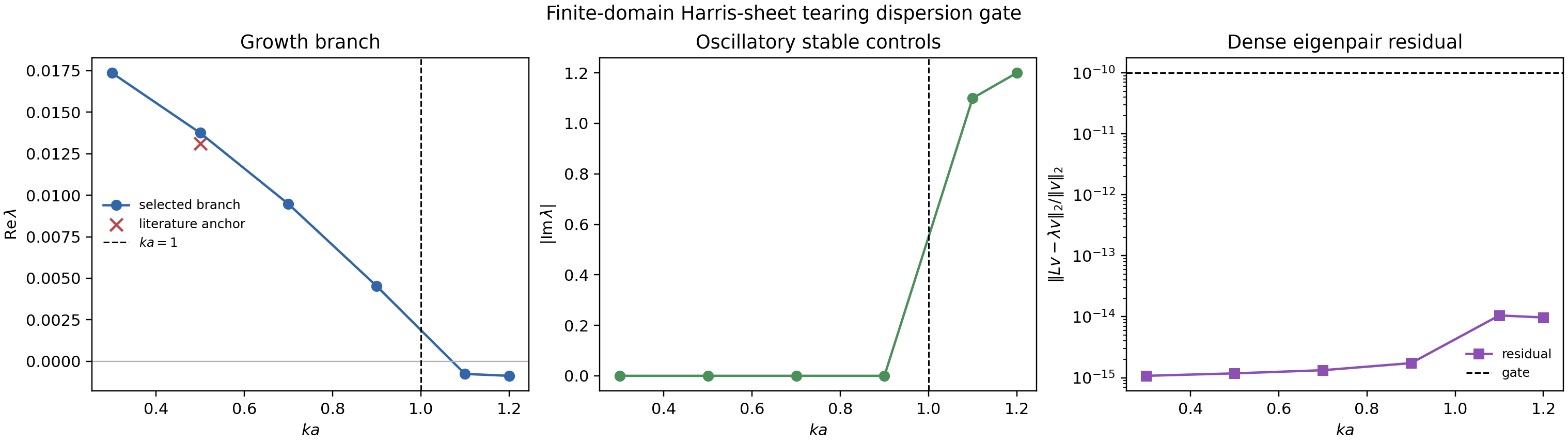
The scan is useful because it catches sign mistakes that a single unstable eigenvalue cannot: the code must recover an unstable tearing band below \(ka=1\) and stable oscillatory controls above \(ka=1\). The remaining research-grade target is a higher-resolution Lundquist-number sweep that separates constant-\(\psi\) FKR and large-\(\Delta'\) Coppi branches.

Harris eigenfunction layer gate

The direct eigenvalue and dispersion gates verify growth rates and residuals. They do not by themselves verify that the selected eigenfunction has the expected resonant-surface localization. MHX therefore adds a conservative FAST shape gate over a Lundquist-number scan. For each sampled \(S\), it solves the same Harris eigenproblem and measures half-maximum widths for:

\[ b(x),\qquad \operatorname{Im}u(x),\qquad j_1(x)=-\left(\frac{d^2}{dx^2}-k^2\right)b(x). \]

The validation gates are deliberately qualitative:

\[ \Delta_u(S_1)>\Delta_u(S_2)>\cdots,\qquad \operatorname{spread}(\Delta_b)/\langle\Delta_b\rangle \ll 1, \]

where \(\Delta_u\) is the flow-layer half-width and \(\Delta_b\) is the outer flux half-width. The fitted slopes are recorded and checked only against broad FAST ranges. They should not be interpreted as production FKR/Coppi exponents.

mhx benchmark linear-tearing-layer \
  --outdir outputs/benchmarks/linear_tearing_layer

Expected files:

• outputs/benchmarks/linear_tearing_layer/diagnostics.json

• outputs/benchmarks/linear_tearing_layer/validation.json

• outputs/benchmarks/linear_tearing_layer/linear_tearing_layer.npz

• outputs/benchmarks/linear_tearing_layer/figures/linear_tearing_layer.png

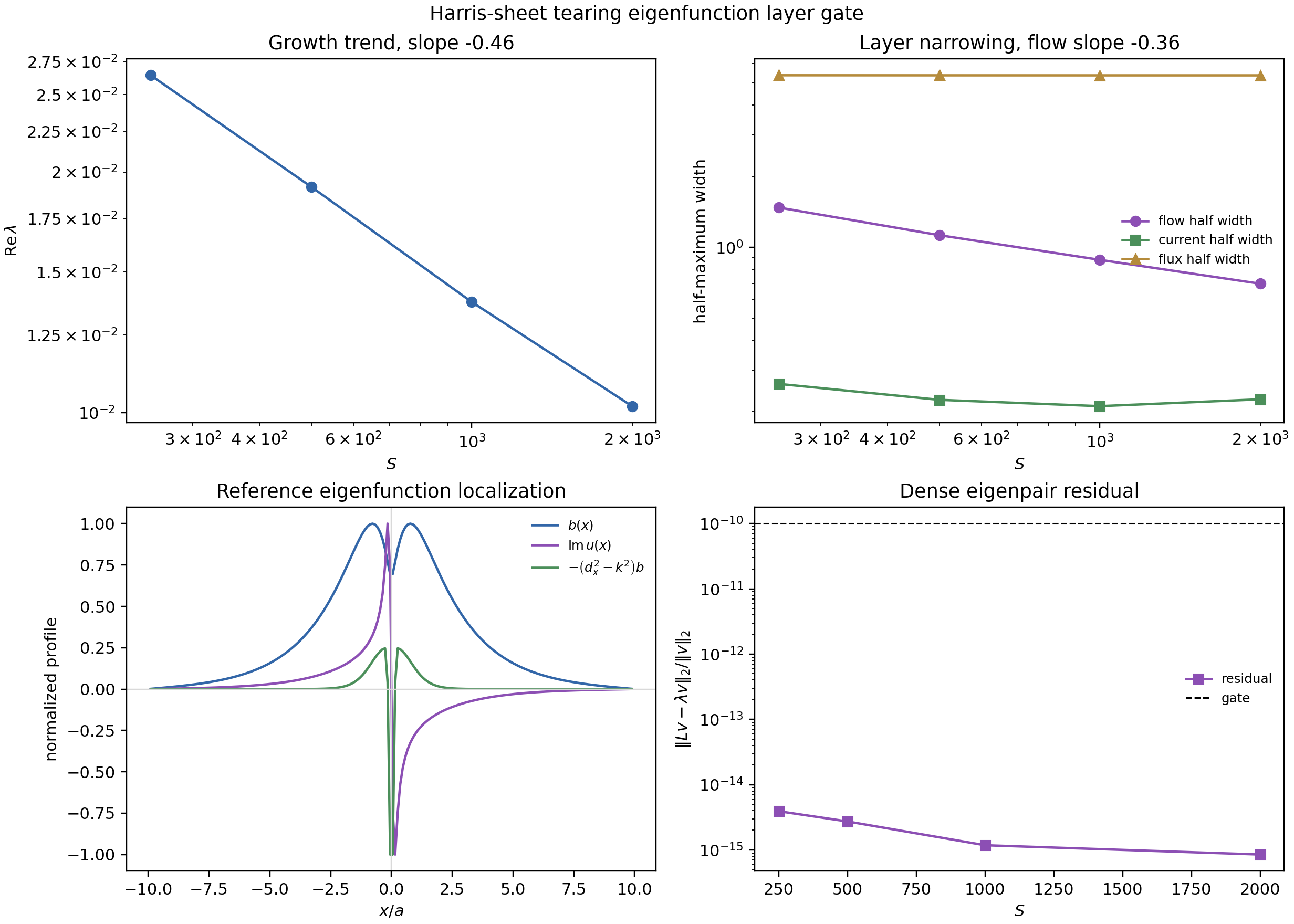
This gate is useful because it catches a different class of failure than a growth-rate check: an implementation can select a plausible eigenvalue while returning a poorly localized or mis-phased eigenfunction. The current gate confirms monotonic narrowing of the flow layer and stability of the outer flux envelope in the FAST scan.

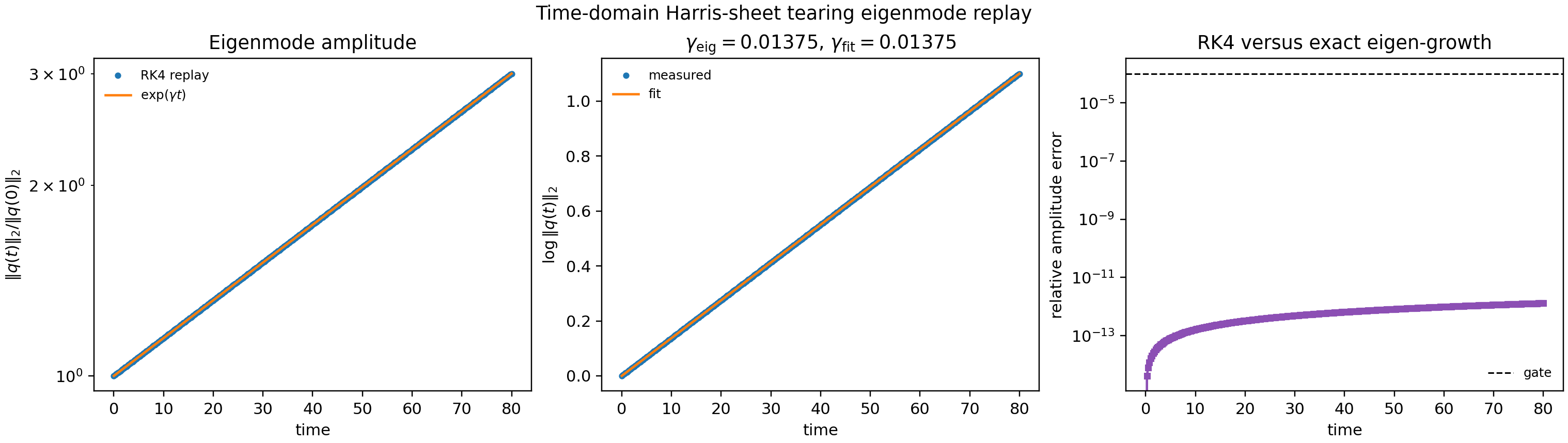
Time-domain Harris eigenmode replay

A growth-rate diagnostic is only useful if it recovers the known rate from a time signal. MHX therefore reuses the same direct Harris-sheet operator \(L\) and selected eigenvector \(q_0\) from the eigenvalue gate, then integrates

\[ \frac{dq}{dt}=Lq,\qquad q(0)=q_0,\qquad Lq_0=\lambda q_0 . \]

For a pure eigenmode,

\[ \|q(t)\|_2 = \|q_0\|_2\exp(\operatorname{Re}\lambda\,t). \]

The benchmark advances the finite-dimensional system with RK4, fits \(\log\|q(t)\|_2\) over the configured window, and gates:

\[ \frac{|\gamma_\mathrm{fit}-\operatorname{Re}\lambda|} {|\operatorname{Re}\lambda|}\le \epsilon_\gamma, \qquad \max_t\frac{|\|q(t)\|_2-\exp(\operatorname{Re}\lambda t)|} {\exp(\operatorname{Re}\lambda t)} \le \epsilon_A . \]

It also verifies that the final state remains aligned with the initial eigenvector. This closes the loop between eigenvalue calculation, time integration, and growth fitting. It is still a linear finite-domain replay; it does not claim nonlinear island growth or saturation.

mhx benchmark linear-tearing-timedomain \
  --outdir outputs/benchmarks/linear_tearing_timedomain

Expected files:

• outputs/benchmarks/linear_tearing_timedomain/diagnostics.json

• outputs/benchmarks/linear_tearing_timedomain/validation.json

• outputs/benchmarks/linear_tearing_timedomain/linear_tearing_timedomain.npz

• outputs/benchmarks/linear_tearing_timedomain/figures/linear_tearing_timedomain.png

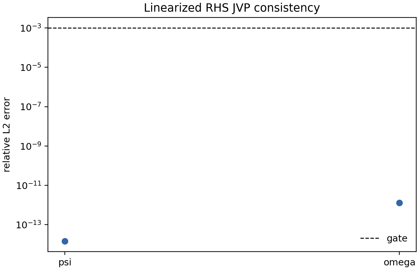
Matrix-free linearized RHS

Tearing eigenmode calculations require a linearized operator \(\mathcal{L}=\partial F/\partial q\) for the reduced-MHD state \(q=(\psi,\omega)\). MHX exposes this as a matrix-free Jacobian-vector product:

\[ \mathcal{L}(q)\,\delta q = \left.\frac{d}{d\epsilon}F(q+\epsilon\delta q)\right|_{\epsilon=0}, \]

computed by JAX forward-mode automatic differentiation. The validation gate compares that JVP against the centered finite-difference approximation

\[ \frac{F(q+\epsilon\delta q)-F(q-\epsilon\delta q)}{2\epsilon}. \]

mhx benchmark linearized-rhs --outdir outputs/benchmarks/linearized_rhs

Expected files:

• outputs/benchmarks/linearized_rhs/diagnostics.json

• outputs/benchmarks/linearized_rhs/validation.json

• outputs/benchmarks/linearized_rhs/linearized_rhs.npz

• outputs/benchmarks/linearized_rhs/figures/linearized_rhs_errors.png

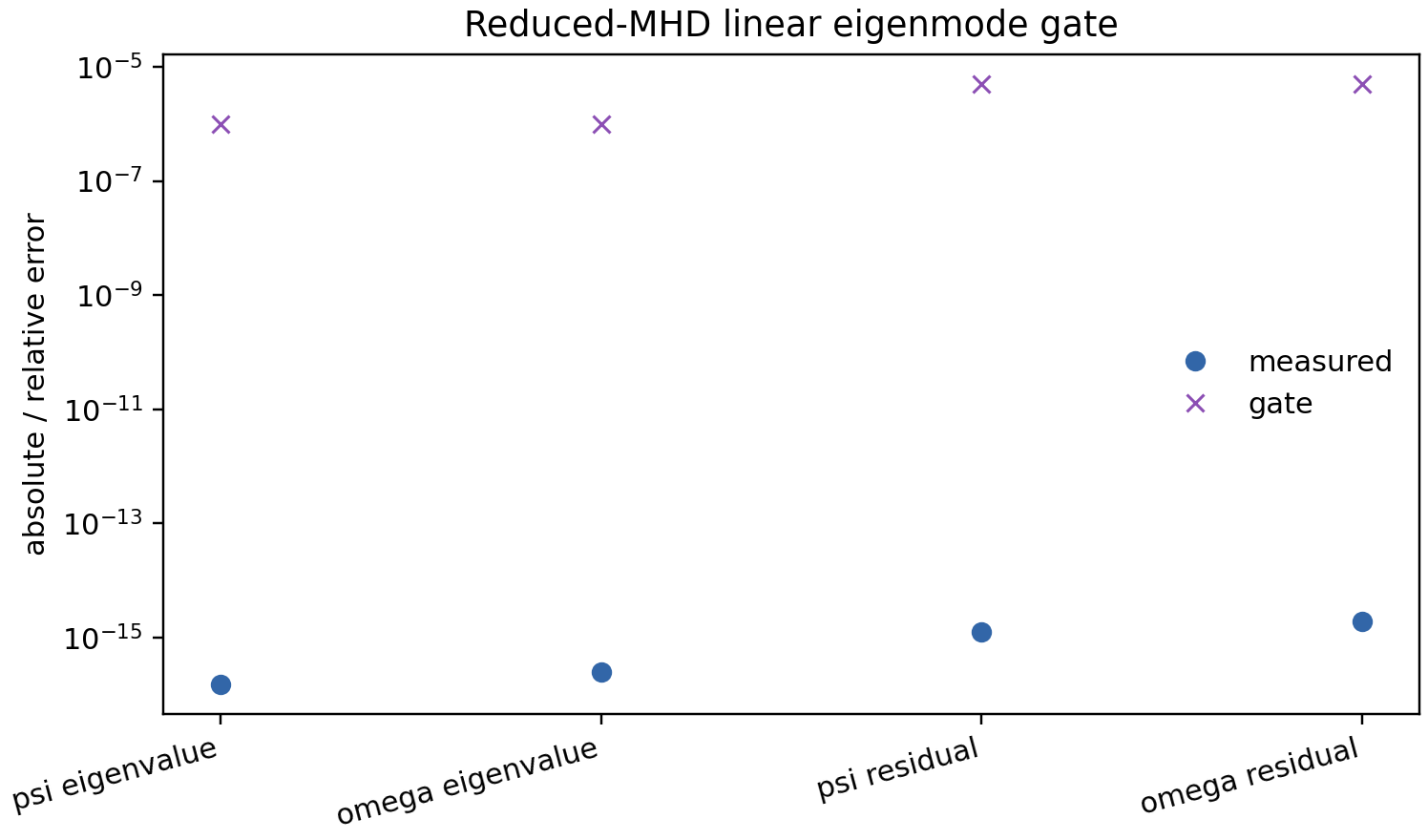
Reduced-MHD linear eigenmode gate

At zero flux and zero flow, the reduced-MHD JVP operator decouples into two Fourier diffusion blocks:

\[ \partial_t\delta\psi = \eta\nabla^2\delta\psi,\qquad \partial_t\delta\omega = \nu\nabla^2\delta\omega. \]

For a periodic Fourier mode \(\sin(k_xx+k_yy)\), the expected eigenvalues are

\[ \lambda_\psi = -\eta(k_x^2+k_y^2),\qquad \lambda_\omega = -\nu(k_x^2+k_y^2). \]

This gate applies linearized_reduced_mhd_operator to flattened \((\delta\psi,\delta\omega)\) vectors and checks Rayleigh quotients and eigen-residuals for both blocks. It is the first physics-facing use of the full flattened reduced-MHD linear operator; nonzero-equilibrium tearing eigenmodes will build on this path.

mhx benchmark reduced-mhd-eigenmode --outdir outputs/benchmarks/reduced_mhd_eigenmode

Expected files:

• outputs/benchmarks/reduced_mhd_eigenmode/diagnostics.json

• outputs/benchmarks/reduced_mhd_eigenmode/validation.json

• outputs/benchmarks/reduced_mhd_eigenmode/reduced_mhd_linear_eigenmode.npz

• outputs/benchmarks/reduced_mhd_eigenmode/figures/reduced_mhd_linear_eigenmode_errors.png

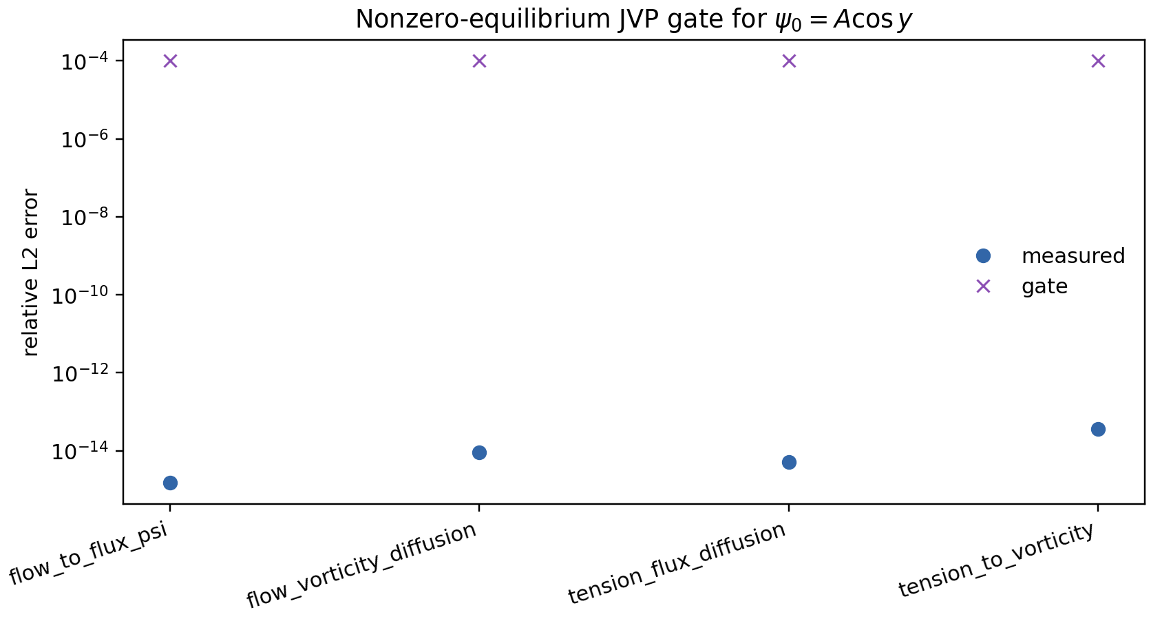
Nonzero cosine-equilibrium linearization gate

This gate validates the linearized operator on a nonzero current-sheet equilibrium before the tearing eigenmode checks below. MHX uses the periodic equilibrium

\[ \psi_0=A\cos(k_y y),\qquad \omega_0=0, \]

and checks exact Poisson-bracket couplings for two perturbations.

First, a pure vorticity perturbation \(\delta\omega=\cos(k_xx)\) gives \(\delta\phi=-\cos(k_xx)/k_x^2\). The flux equation contains flow advection of the equilibrium field:

\[ \partial_t\delta\psi =-[\delta\phi,\psi_0] =A\frac{k_y}{k_x}\sin(k_xx)\sin(k_yy), \qquad \partial_t\delta\omega=-\nu k_x^2\cos(k_xx). \]

Second, a pure flux perturbation \(\delta\psi=\cos(k_xx)\cos(2k_yy)\) checks magnetic tension:

\[ \partial_t\delta\omega =[\delta\psi,\nabla^2\psi_0]+[\psi_0,\nabla^2\delta\psi] =A k_x k_y (k_x^2+4k_y^2-k_y^2) \sin(k_xx)\sin(k_yy)\cos(2k_yy), \]

while the flux block diffuses as

\[ \partial_t\delta\psi=-\eta(k_x^2+4k_y^2)\delta\psi. \]

This gate does not claim an FKR growth rate. It validates the exact nonzero equilibrium coupling terms that the FKR/plasmoid eigenmode benchmarks will depend on.

mhx benchmark cosine-equilibrium-linearization \
  --outdir outputs/benchmarks/cosine_equilibrium_linearization

Expected files:

• outputs/benchmarks/cosine_equilibrium_linearization/diagnostics.json

• outputs/benchmarks/cosine_equilibrium_linearization/validation.json

• outputs/benchmarks/cosine_equilibrium_linearization/cosine_equilibrium_linearization.npz

• outputs/benchmarks/cosine_equilibrium_linearization/figures/cosine_equilibrium_linearization_errors.png

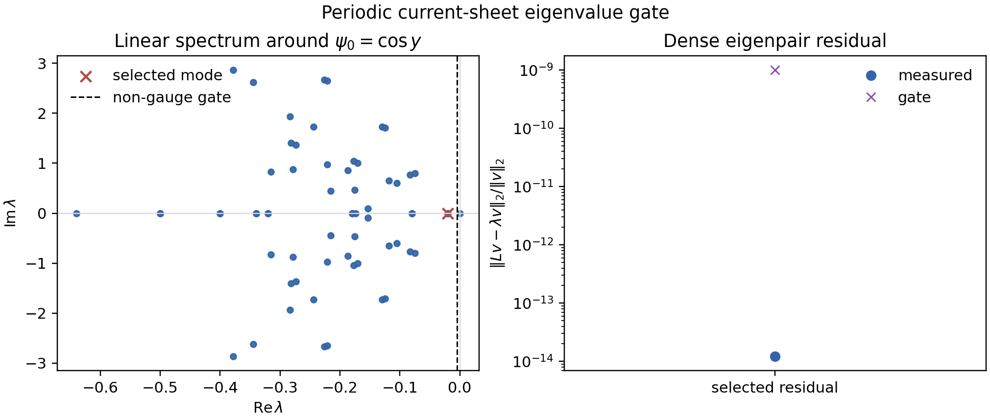
Periodic current-sheet eigenvalue gate

The first nonzero-equilibrium spectrum gate now assembles the full flattened JVP matrix on a deliberately tiny grid for

\[ \psi_0=A\cos(2\pi y/L_y),\qquad \omega_0=0. \]

This is still not an FKR/Coppi growth-rate claim. It is a conservative operator-stability gate between exact bracket tests and future asymptotic tearing benchmarks. The benchmark checks:

\[ \|L\,\mathbf{1}_\psi\|_2 \approx 0,\qquad \|L\,\mathbf{1}_\omega\|_2 \approx 0, \]

for the two mean/gauge modes, solves the complete dense spectrum, and requires the non-gauge spectrum to be damped:

\[ \max_{\lambda\notin\mathrm{gauge}}\operatorname{Re}\lambda \le -c\,\min(\eta,\nu)\,k_{\min}^2, \]

with \(c=0.25\) in the FAST gate. It also stores the selected dense eigenpair and checks the residual

\[ \frac{\|Lv-\lambda v\|_2}{\|v\|_2} \]

against a tight x64 tolerance.

mhx benchmark current-sheet-eigenvalue \
  --outdir outputs/benchmarks/periodic_current_sheet_eigenvalue

Expected files:

• outputs/benchmarks/periodic_current_sheet_eigenvalue/diagnostics.json

• outputs/benchmarks/periodic_current_sheet_eigenvalue/validation.json

• outputs/benchmarks/periodic_current_sheet_eigenvalue/periodic_current_sheet_eigenvalue.npz

• outputs/benchmarks/periodic_current_sheet_eigenvalue/figures/periodic_current_sheet_spectrum.png

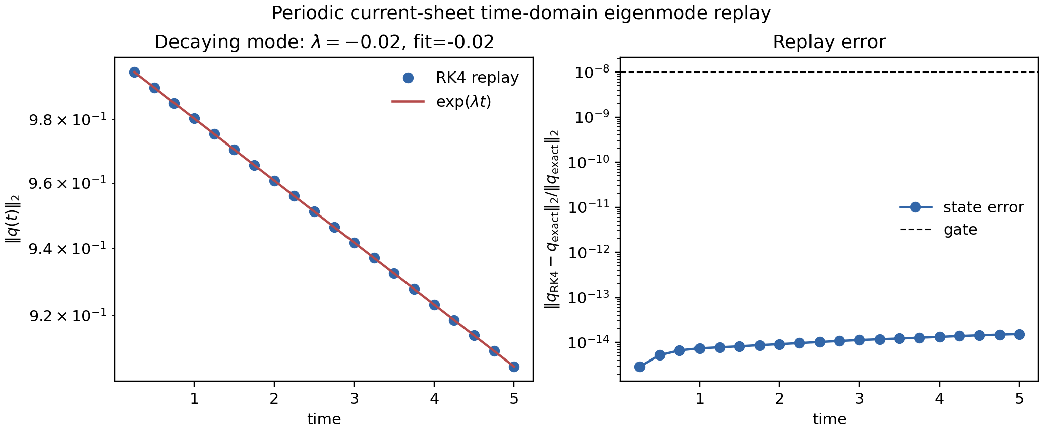
Periodic current-sheet time-domain replay

The dense spectrum gate proves that the assembled periodic current-sheet JVP has the expected gauge modes and a damped non-gauge spectrum on the FAST grid. The time-domain replay adds the next solver-level check: select a real decaying eigenmode of the same operator and integrate

\[ \frac{d q}{dt}=Lq,\qquad q(0)=v,\qquad Lv=\lambda v. \]

For this linear initial value problem the exact solution is

\[ q(t)=e^{\lambda t}v . \]

The benchmark advances \(q\) with the RK4 path used by MHX validation workflows, then gates both the full state-vector error and the decay-rate fit from \(\log\|q(t)\|_2\):

\[ \epsilon_q(t)=\frac{\|q_{\mathrm{RK4}}(t)-e^{\lambda t}v\|_2} {\|e^{\lambda t}v\|_2},\qquad \gamma_{\mathrm{fit}}\approx \lambda . \]

This is deliberately a linear operator/time-step bridge, not a nonlinear magnetic-island or FKR/Coppi tearing-growth claim.

mhx benchmark current-sheet-timedomain \
  --outdir outputs/benchmarks/periodic_current_sheet_timedomain

Expected files:

• outputs/benchmarks/periodic_current_sheet_timedomain/diagnostics.json

• outputs/benchmarks/periodic_current_sheet_timedomain/validation.json

• outputs/benchmarks/periodic_current_sheet_timedomain/periodic_current_sheet_timedomain.npz

• outputs/benchmarks/periodic_current_sheet_timedomain/figures/periodic_current_sheet_timedomain.png

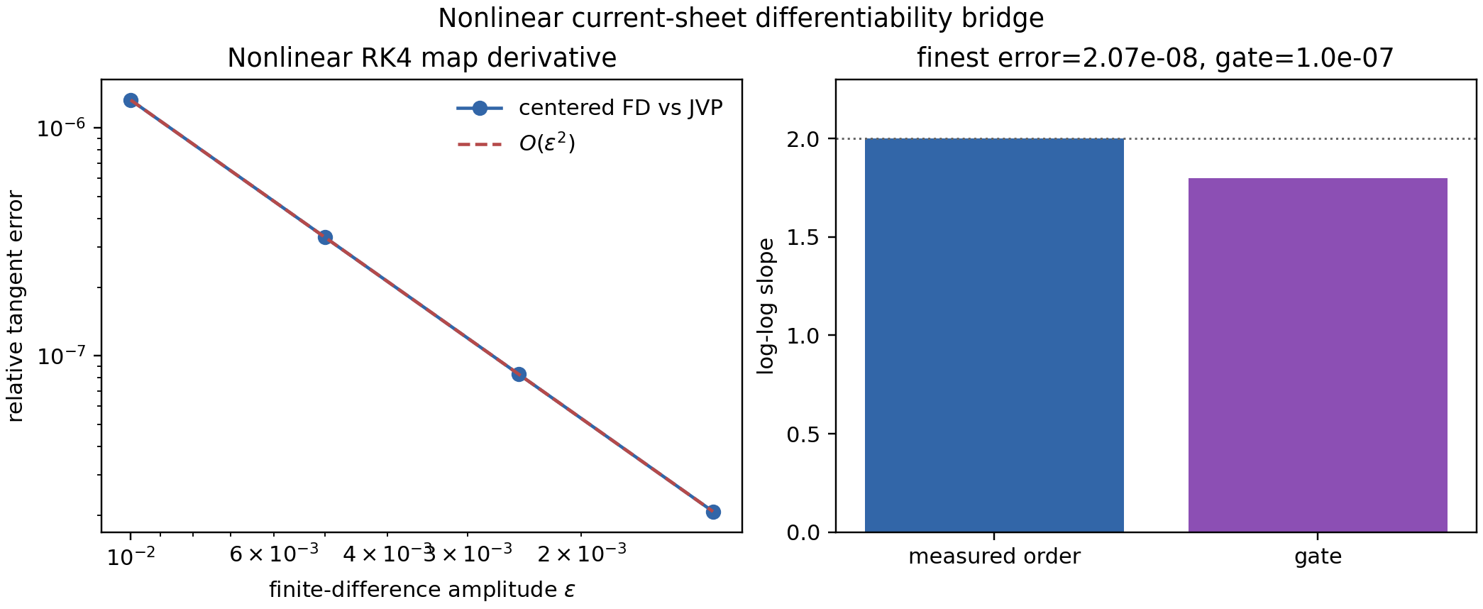
Nonlinear current-sheet differentiability bridge

The linear replay gate validates a frozen operator. The next differentiable solver gate validates the nonlinear RK4 time map used by actual MHX runs. Let \(\Phi(q_0)\) be the map from an initial reduced-MHD state to the saved trajectory vector after several RK4 steps. Around the periodic current sheet \(q_0=(\psi_0,\omega_0)\), JAX gives a tangent

\[ \delta \Phi = D\Phi(q_0)[p]. \]

MHX compares that tangent to centered finite differences of full nonlinear trajectories:

\[ \delta \Phi_\epsilon = \frac{\Phi(q_0+\epsilon p)-\Phi(q_0-\epsilon p)}{2\epsilon}. \]

For a smooth RHS and x64 arithmetic, the error should converge as

\[ \frac{\|\delta \Phi_\epsilon-\delta\Phi\|_2}{\|\delta\Phi\|_2} = O(\epsilon^2) \]

until roundoff. This gate is specifically aimed at differentiable programming claims: before MHX trains neural ODEs, adjoints, or inverse-design loops on solver trajectories, the trajectory map itself must have a verified tangent.

mhx benchmark current-sheet-nonlinear-bridge \
  --outdir outputs/benchmarks/periodic_current_sheet_nonlinear_bridge

Expected files:

• outputs/benchmarks/periodic_current_sheet_nonlinear_bridge/diagnostics.json

• outputs/benchmarks/periodic_current_sheet_nonlinear_bridge/validation.json

• outputs/benchmarks/periodic_current_sheet_nonlinear_bridge/periodic_current_sheet_nonlinear_bridge.npz

• outputs/benchmarks/periodic_current_sheet_nonlinear_bridge/figures/periodic_current_sheet_nonlinear_bridge.png

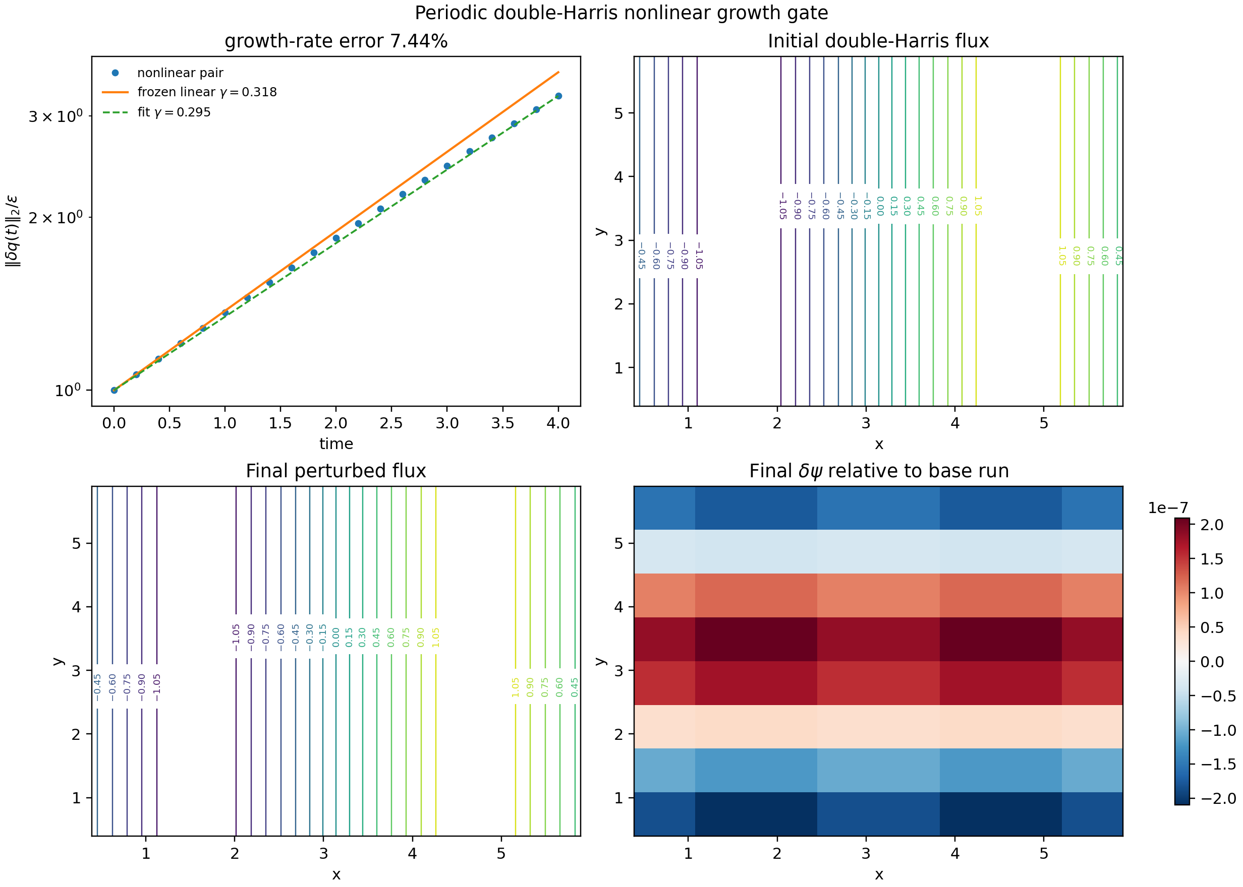
Periodic double-Harris nonlinear growth gate

The stable cosine-current-sheet spectrum above is intentionally conservative: it protects the code from spurious positive growth but does not demonstrate tearing. MHX now adds a small-grid instability gate using a periodic double-Harris sheet,

\[ B_y(x)=A\left[\tanh\left(\frac{x-L_x/4}{a}\right) -\tanh\left(\frac{x-3L_x/4}{a}\right)-1\right], \]

with a zero-mean flux \(\psi_0\) satisfying \(B_y=\partial_x\psi_0\) to the sign convention used by the reduced-MHD solver. The gate assembles the dense matrix-free Jacobian \(L=D F(\psi_0,0)\), selects the fastest non-gauge unstable eigenmode \(Lv=\gamma v\), and advances two full nonlinear trajectories:

\[ q_b(t)=\Phi_t(q_0),\qquad q_p(t)=\Phi_t(q_0+\epsilon v). \]

The measured finite-amplitude difference

\[ A(t)=\frac{\|q_p(t)-q_b(t)\|_2}{\epsilon} \]

must grow by more than a factor of two and its fitted rate must remain within a documented tolerance of the frozen-base eigenvalue. This is the first MHX validation artifact that shows a physically unstable current sheet growing in the nonlinear solver. It is still not a Rutherford-island or plasmoid-chain production claim: the grid is deliberately tiny, the base sheet is periodic, and publication claims still require duration, resolution, time-step, seed, and aspect-ratio sweeps. The literature anchors are the classical tearing-mode instability of Furth–Killeen–Rosenbluth (Physics of Fluids 6, 459, 1963) and the high-Lundquist-number plasmoid-chain scalings of Loureiro–Schekochihin–Cowley (arXiv:astro-ph/0703631), with later nonlinear plasmoid-chain simulations by Samtaney et al. (arXiv:0903.0542).

mhx benchmark double-harris-growth \
  --outdir outputs/benchmarks/periodic_double_harris_nonlinear_growth

Expected files:

• outputs/benchmarks/periodic_double_harris_nonlinear_growth/diagnostics.json

• outputs/benchmarks/periodic_double_harris_nonlinear_growth/validation.json

• outputs/benchmarks/periodic_double_harris_nonlinear_growth/periodic_double_harris_nonlinear_growth.npz

• outputs/benchmarks/periodic_double_harris_nonlinear_growth/figures/periodic_double_harris_nonlinear_growth.png

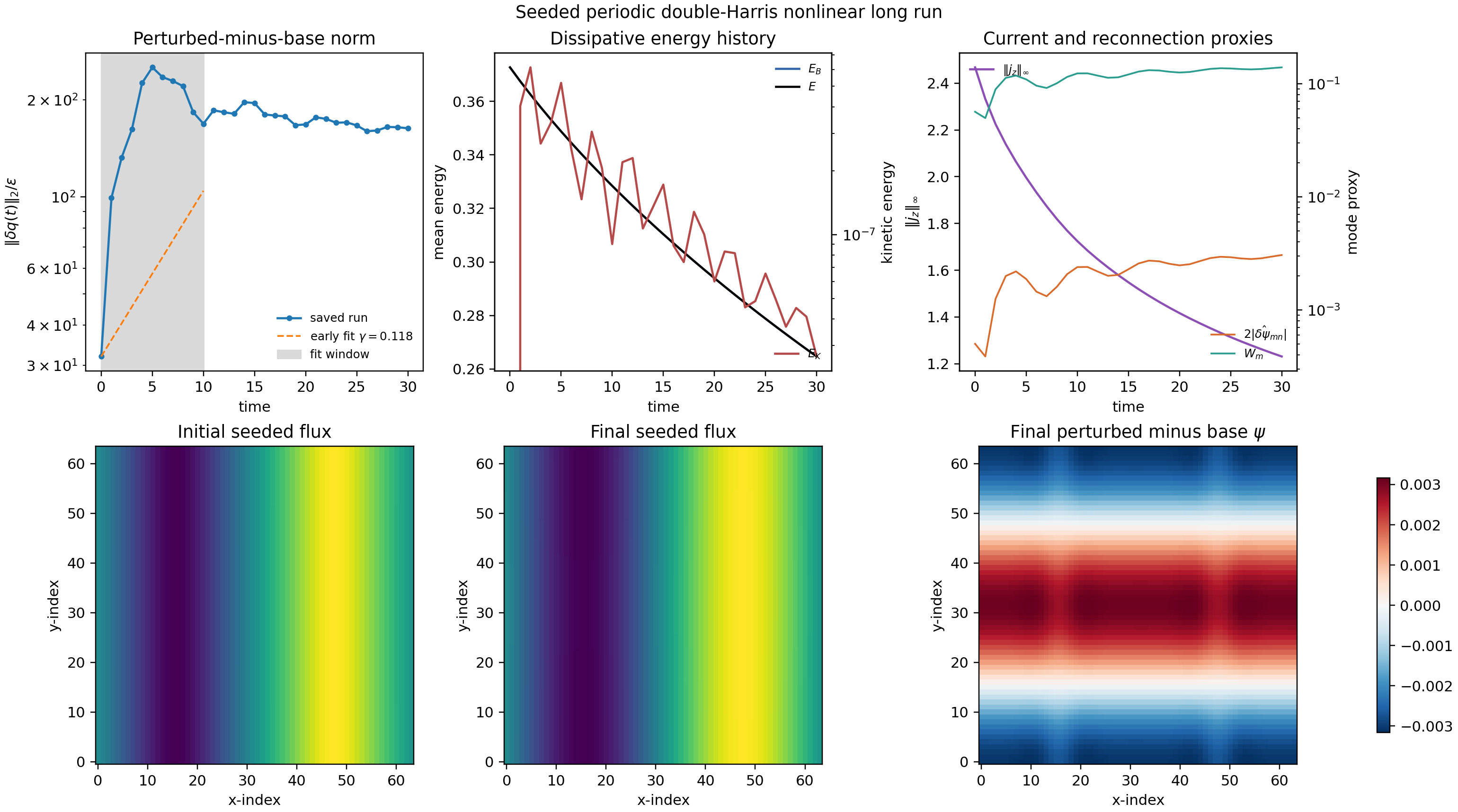
Seeded double-Harris long-run validation

The dense eigenmode gate above is intentionally tiny because it assembles the full Jacobian. The next bridge is a scalable nonlinear run that does not assemble the dense spectrum. It advances a base periodic double-Harris sheet and a seeded sheet,

\[ q_b(t)=\Phi_t(q_0),\qquad q_s(t)=\Phi_t(q_0+\epsilon\cos(2x)\cos y), \]

and tracks the normalized difference, dominant reconnecting-flux proxy, local Rutherford-width proxy, total energy, kinetic energy, peak current density, and X/O critical-point counts:

\[ A_s(t)=\frac{\|q_s(t)-q_b(t)\|_2}{\epsilon},\qquad \psi_\mathrm{rec}(t)=2\max_{0<|k_i|\le N_i/4}|\widehat{\delta\psi}_k(t)|, \qquad W_m(t)=4\sqrt{\frac{|\psi_\mathrm{rec}(t)|}{|A|/a}}, \qquad E(t)=\frac{1}{2}\langle |\nabla\psi|^2+|\nabla\phi|^2\rangle,\qquad \|j_z\|_\infty=\|-\nabla^2\psi\|_\infty . \]

This command is meant for bounded nonlinear evidence runs under laptop/CI budgets and for producing reviewer-visible movies before a full production campaign. It gates finite histories, full-duration completion, an early-time growth fit, visible maximum amplification, and dissipative total-energy behavior. The reconnection proxy is deliberately stated as a dominant low-mode perturbation-flux diagnostic for periodic double-Harris validation: the configured seed-mode amplitude is archived separately as seed_mode_reconnected_flux, so mode transfer is visible rather than hidden. The committed 64×64, t_end=30 evidence bundle gives gamma_early = 0.118, early amplification 5.27×, maximum amplification 7.89×, and zero measured total-energy increase. The result is stronger than a smoke test, but it remains a validation artifact rather than a converged Rutherford/plasmoid claim because the late-time perturbation saturates/relaxes and no resolution/seed/aspect-ratio sweep has yet closed.

mhx benchmark double-harris-long-run \
  --outdir outputs/benchmarks/periodic_double_harris_seeded_long_run \
  --nx 64 --ny 64 --t-end 30 --save-every 100 --movies

Expected files:

• outputs/benchmarks/periodic_double_harris_seeded_long_run/diagnostics.json

• outputs/benchmarks/periodic_double_harris_seeded_long_run/validation.json

• outputs/benchmarks/periodic_double_harris_seeded_long_run/periodic_double_harris_seeded_long_run.npz

• outputs/benchmarks/periodic_double_harris_seeded_long_run/figures/periodic_double_harris_seeded_long_run.png

• outputs/benchmarks/periodic_double_harris_seeded_long_run/figures/periodic_double_harris_flux.gif

• outputs/benchmarks/periodic_double_harris_seeded_long_run/figures/periodic_double_harris_current.gif

Once a convergence bundle exists, the promotion-boundary report is:

mhx benchmark double-harris-promotion-check \
  outputs/benchmarks/periodic_double_harris_seeded_long_run \
  --convergence-dir outputs/benchmarks/periodic_double_harris_convergence

This writes promotion/promotion_readiness.json, promotion/validation.json, and promotion/figures/promotion_matrix.png. Passing means the run is convergence-backed validation evidence; it still does not authorize Rutherford, Sweet–Parker, or plasmoid production claims.

Source anchors:

• double-Harris equilibrium

• growth and long-run benchmark implementation

• growth benchmark tests

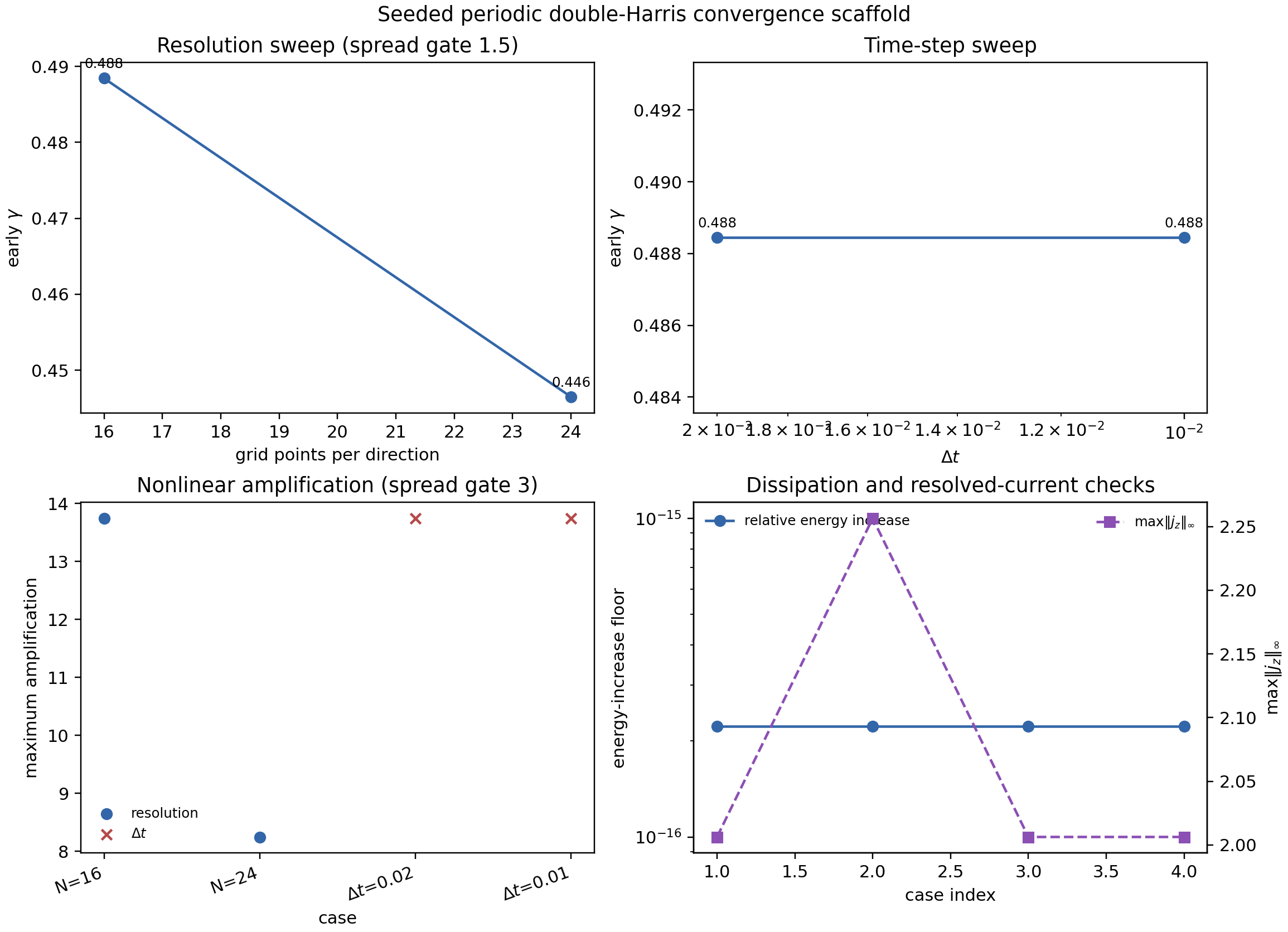
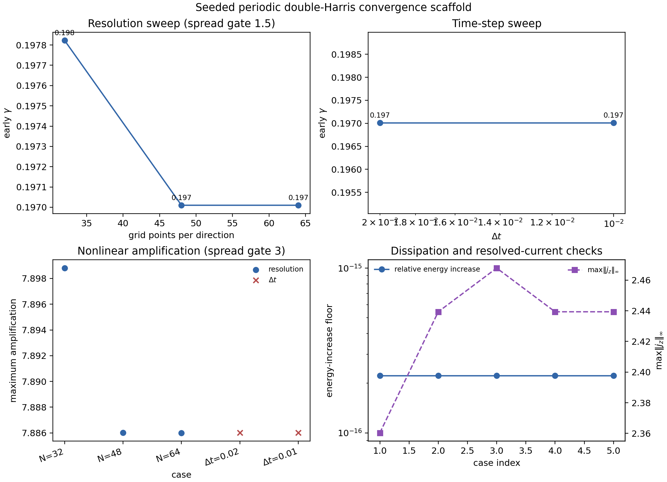
Seeded double-Harris convergence evidence

This gate asks whether the measured early growth and nonlinear amplification are artifacts of one tiny grid or one RK4 step size. The command

mhx benchmark double-harris-convergence \
  --outdir outputs/benchmarks/periodic_double_harris_convergence \
  --resolutions 16,24 --dt-values 0.02,0.01 \
  --reference-resolution 16 --t-end 8 --fit-stop 4

runs the same base-vs-seeded replay across a small resolution sweep and a small time-step sweep. For each case it records

\[ \gamma_\mathrm{fit},\quad G_\mathrm{early}=A_s(t_b)/A_s(t_a),\quad G_\mathrm{max}=\max_t A_s(t)/A_s(0),\quad \Delta E_+=\max_t(E(t)-E(0))_+/E(0). \]

The gate requires finite metrics, positive early growth, dissipative total energy, successful subcase gates, and bounded relative spread in gamma_fit/G_max. The same code path has also been exercised on a GPU-assisted medium sweep with resolutions 32,48,64, t_end=16, and 0.41% growth-rate spread. This is intentionally validation evidence, not a production claim: it prevents single-run overclaiming before larger aspect-ratio, Lundquist-number, seed, and duration sweeps are executed.

Expected files:

• outputs/benchmarks/periodic_double_harris_convergence/diagnostics.json

• outputs/benchmarks/periodic_double_harris_convergence/validation.json

• outputs/benchmarks/periodic_double_harris_convergence/periodic_double_harris_convergence.npz

• outputs/benchmarks/periodic_double_harris_convergence/figures/periodic_double_harris_convergence.png

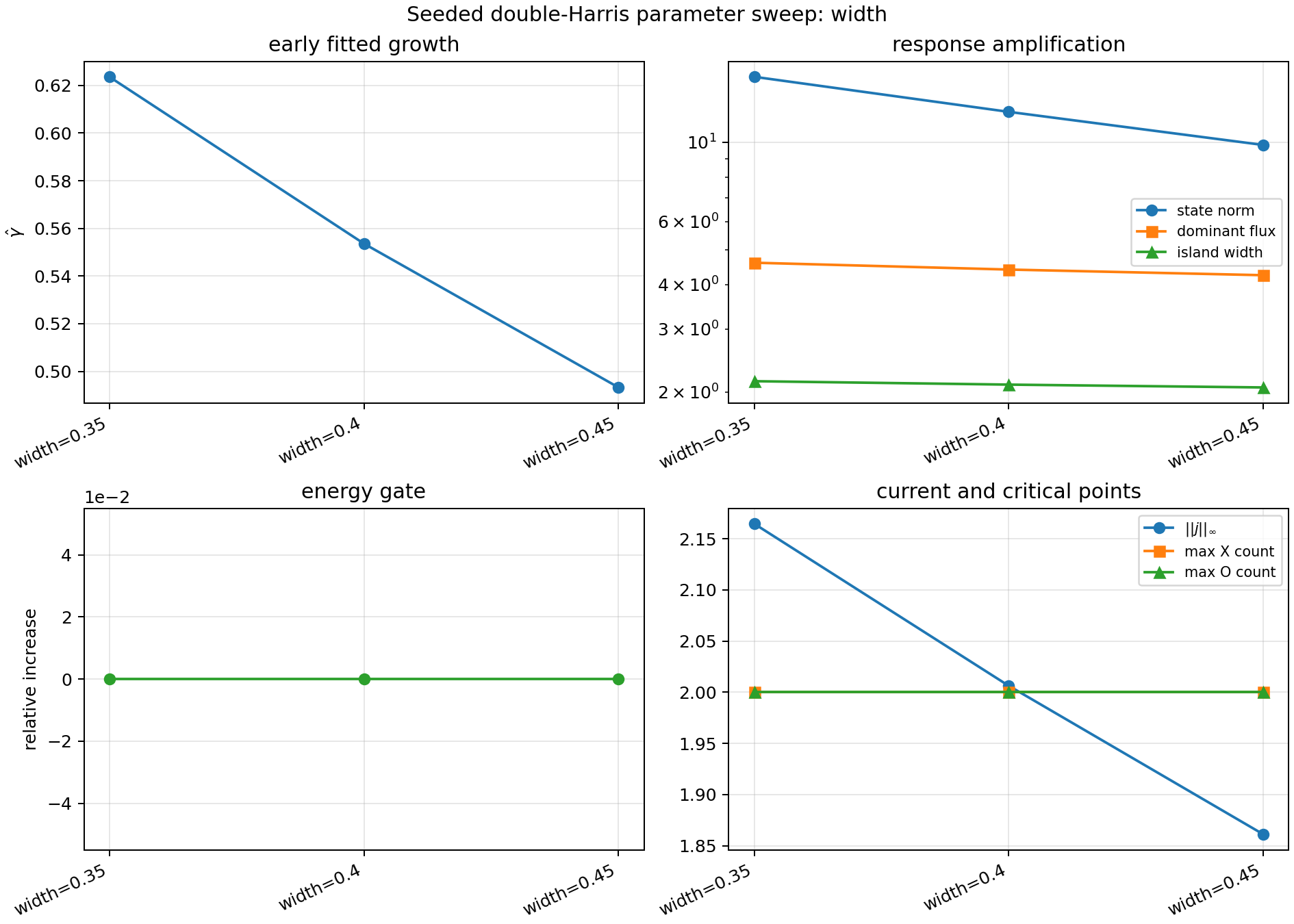
Seeded double-Harris parameter sweeps

Convergence sweeps ask whether one numerical setting dominates the result. Parameter sweeps ask a different question: do the nonlinear response diagnostics remain finite, dissipative, and visibly reconnecting when the seed mode, sheet width, or resistivity is changed? The command

mhx benchmark double-harris-parameter-sweep \
  --outdir outputs/benchmarks/periodic_double_harris_parameter_sweep \
  --sweep-axis width --widths 0.35,0.4,0.45 \
  --t-end 6 --fit-stop 3

runs three seeded base-vs-perturbed replays and records

\[ \gamma_\mathrm{fit},\quad G_\mathrm{max},\quad G_\psi=\max_t \psi_\mathrm{rec}(t)/\psi_\mathrm{rec}(0),\quad G_W=\max_t W(t)/W(0),\quad \Delta E_+ . \]

The gate requires all cases to pass the underlying seeded-long-run checks, and also requires finite per-case metrics, at least three cases, positive fitted growth, visible amplification, reconnecting-flux and island-width response, dissipative total energy, and bounded anomaly-scale spreads. The spread gates are deliberately loose because physically different sheets need not agree; they catch runaway or degenerate cases before figures are promoted.

Expected files:

• outputs/benchmarks/periodic_double_harris_parameter_sweep/diagnostics.json

• outputs/benchmarks/periodic_double_harris_parameter_sweep/validation.json

• outputs/benchmarks/periodic_double_harris_parameter_sweep/periodic_double_harris_parameter_sweep.npz

• outputs/benchmarks/periodic_double_harris_parameter_sweep/figures/periodic_double_harris_parameter_sweep.png

Source anchors:

• convergence runner

• convergence CLI

• convergence tests

Nonlinear reduced-MHD energy budget

The first full nonlinear PDE gate is deliberately not a plasmoid claim. It checks the periodic reduced-MHD energy theorem under the complete nonlinear Poisson-bracket RHS. For

\[ E(t)=\frac{1}{2}\left\langle |\nabla\psi|^2+|\nabla\phi|^2\right\rangle, \qquad \nabla^2\phi=\omega,\qquad j=-\nabla^2\psi, \]

periodic integration by parts gives

\[ \frac{dE}{dt}=-\eta\langle j^2\rangle-\nu\langle\omega^2\rangle. \]

This identity is a strong nonlinear sign/cancellation check: the advection and magnetic-tension brackets must cancel in the energy balance, while the resistive and viscous terms must remove energy. MHX starts from a multi-mode state with active nonlinear RHS, advances the full nonlinear RK4 solver, and gates:

• all saved arrays are finite;

• the initial nonlinear RHS norm is a nontrivial fraction of the full RHS;

• total energy is nonincreasing;

• the integrated residual \(|E(t)-E(0)+\int_0^t[\eta\langle j^2\rangle+\nu\langle\omega^2\rangle]dt|/E(0)\) stays below tolerance;

• net dissipative energy loss is observed.

mhx benchmark nonlinear-energy-budget \
  --outdir outputs/benchmarks/nonlinear_energy_budget

Expected files:

• outputs/benchmarks/nonlinear_energy_budget/diagnostics.json

• outputs/benchmarks/nonlinear_energy_budget/validation.json

• outputs/benchmarks/nonlinear_energy_budget/nonlinear_energy_budget.npz

• outputs/benchmarks/nonlinear_energy_budget/figures/nonlinear_energy_budget.png

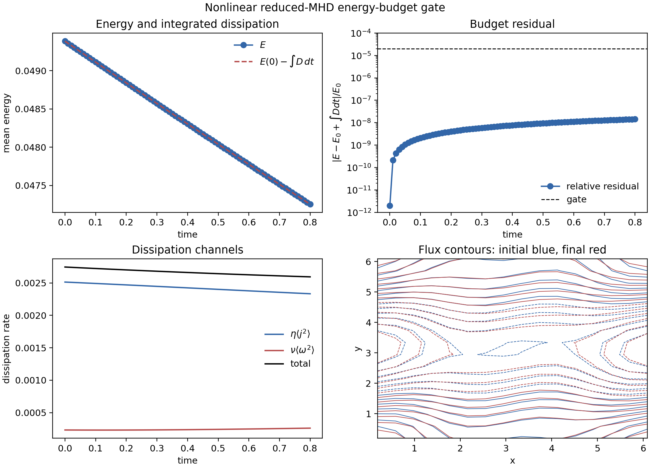
This is the most important nonlinear solver gate currently in MHX. It supports claims about nonlinear reduced-MHD consistency, but it still does not validate nonlinear island growth, Rutherford saturation, Sweet–Parker reconnection rates, or plasmoid chains.

Nonlinear duration audit

The nonlinear energy-budget gate is intentionally short. To prevent accidental overclaiming, MHX includes a reviewer-facing duration audit. For a linear tearing eigenmode with growth rate \(\gamma\), observing \(N_e\) e-folds requires

\[ t_\mathrm{end}\ge \frac{N_e}{\gamma}. \]

Using the direct Harris benchmark anchor \(\gamma\simeq0.0131\) for \(S=1000\), \(ka=0.5\), ten e-folds require \(t_\mathrm{end}\approx763.4\). The default FAST nonlinear budget run reaches \(t=0.8\), so it is a code-validity gate, not a nonlinear island or plasmoid physics result. Longer validation runs are documented separately and still require convergence and seed-QI promotion evidence before supporting production physics claims. The audit also records Loureiro-type Sweet–Parker plasmoid one-e-fold estimates \(1/\gamma_{\max}\sim S^{-1/4}\) as a separate linear-timescale reference.

mhx benchmark nonlinear-duration-audit \
  --outdir outputs/benchmarks/nonlinear_duration_audit

Expected files:

• outputs/benchmarks/nonlinear_duration_audit/diagnostics.json

• outputs/benchmarks/nonlinear_duration_audit/validation.json

• outputs/benchmarks/nonlinear_duration_audit/nonlinear_duration_audit.npz

• outputs/benchmarks/nonlinear_duration_audit/figures/nonlinear_duration_audit.png

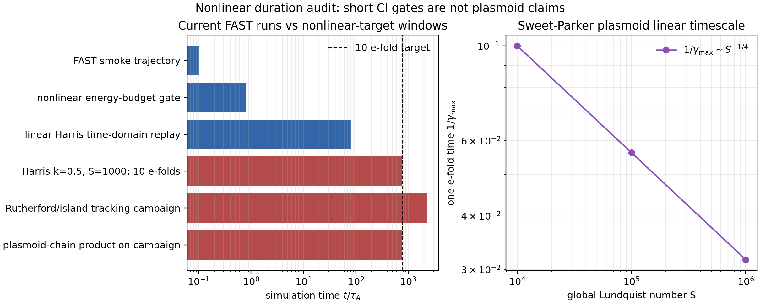
This audit is a pass/fail gate on scientific honesty: it passes only when the current FAST nonlinear runs are explicitly flagged as too short for Rutherford-island or plasmoid-chain claims and when the production time windows are recorded in machine-readable artifacts.

Duration-policy gate

The duration audit is the figure-facing view. The duration-policy gate is the machine-readable rule that future production workflows should call before launching long nonlinear runs:

mhx benchmark duration-policy --outdir outputs/benchmarks/duration_policy

Expected files:

• outputs/benchmarks/duration_policy/duration_policy.json

• outputs/benchmarks/duration_policy/duration_policy.md

• outputs/benchmarks/duration_policy/validation.json

• outputs/benchmarks/duration_policy/manifest.json

The policy gate passes when short historical/CI runs are scoped as validation-only and when future production templates satisfy \(t_\mathrm{end}\ge s_f N_e/\gamma\). This prevents a future script from silently using a smoke-test time window for a nonlinear reconnection claim.

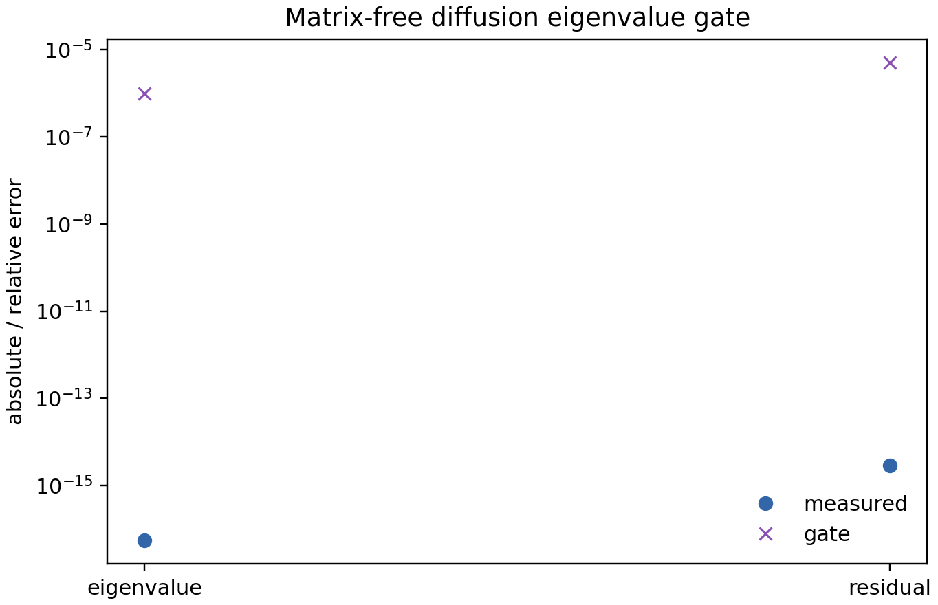
Diffusion eigenvalue scaffold

Before applying eigenvalue machinery to tearing equilibria, MHX validates the matrix-free operator path on a single Fourier eigenfunction of the periodic diffusion operator:

\[ \mathcal{D}\psi = \eta\nabla^2\psi,\qquad \psi_k=\sin(k_x x+k_y y),\qquad \lambda_k = -\eta(k_x^2+k_y^2). \]

The benchmark computes the Rayleigh quotient

\[ \lambda_{\mathrm{RQ}} = \frac{\langle \psi_k,\mathcal{D}\psi_k\rangle} {\langle \psi_k,\psi_k\rangle}, \]

and the relative eigen-residual

\[ \frac{\|\mathcal{D}\psi_k-\lambda_k\psi_k\|_2}{\|\psi_k\|_2}. \]

mhx benchmark diffusion-eigenvalue --outdir outputs/benchmarks/diffusion_eigenvalue

Expected files:

• outputs/benchmarks/diffusion_eigenvalue/diagnostics.json

• outputs/benchmarks/diffusion_eigenvalue/validation.json

• outputs/benchmarks/diffusion_eigenvalue/diffusion_eigenvalue.npz

• outputs/benchmarks/diffusion_eigenvalue/figures/diffusion_eigenvalue_errors.png

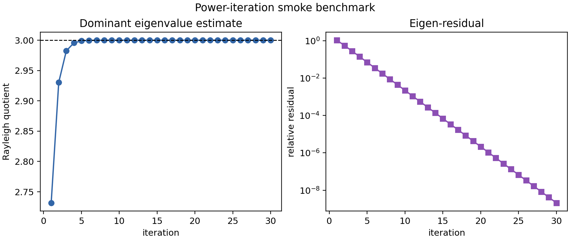
Power-iteration scaffold

The next eigenvalue-control-path gate validates the dominant-eigenpair iteration on a diagonal matrix-free operator

\[ \mathcal{A}u = \operatorname{diag}(3,-1.5,0.5,0.1)u, \]

whose dominant eigenvalue is known exactly:

\[ \lambda_\star = 3. \]

Power iteration repeatedly applies

\[ u_{n+1}=\frac{\mathcal{A}u_n}{\|\mathcal{A}u_n\|_2}, \]

and records the Rayleigh quotient

\[ \lambda_n = \frac{\langle u_n,\mathcal{A}u_n\rangle}{\langle u_n,u_n\rangle} \]

plus residual \(\|\mathcal{A}u_n-\lambda_nu_n\|_2\). This is intentionally a known finite-dimensional operator, not a tearing benchmark. It makes the dominant-eigenpair loop, convergence history, plotting, schemas, CLI, and CI artifact checks deterministic before coupling the same machinery to the reduced-MHD JVP operator.

mhx benchmark power-iteration --outdir outputs/benchmarks/power_iteration

Expected files:

• outputs/benchmarks/power_iteration/diagnostics.json

• outputs/benchmarks/power_iteration/validation.json

• outputs/benchmarks/power_iteration/power_iteration_history.npz

• outputs/benchmarks/power_iteration/figures/power_iteration_history.png

Arnoldi Ritz-spectrum scaffold

Tearing eigenmode validation needs more than a dominant-mode iteration: the linearized reduced-MHD operator can be non-normal, and nearby Ritz values must be handled explicitly. MHX therefore includes a deterministic Arnoldi gate on a small non-normal upper-triangular fixture,

\[\begin{split} \mathcal{A} = \begin{bmatrix} 2 & 0.4 & 0 & 0 \\ 0 & 1 & 0.1 & 0 \\ 0 & 0 & -0.5 & 0.2 \\ 0 & 0 & 0 & 0.1 \end{bmatrix}, \end{split}\]

whose exact spectrum is the diagonal:

\[ \sigma(\mathcal{A}) = \{2, 1, -0.5, 0.1\}. \]

The Arnoldi process constructs an orthonormal Krylov basis \(Q_m\) and projected Hessenberg matrix \(H_m\),

\[ \mathcal{A}Q_m = Q_mH_m + h_{m+1,m}q_{m+1}e_m^\top. \]

The eigenvalues of \(H_m\) are Ritz values approximating the spectrum of \(\mathcal{A}\). The validation gate checks the recovered fixture spectrum, negligible imaginary parts for this real fixture, and residual estimates \(|h_{m+1,m}e_m^\top y_i|\).

mhx benchmark arnoldi --outdir outputs/benchmarks/arnoldi

Expected files:

• outputs/benchmarks/arnoldi/diagnostics.json

• outputs/benchmarks/arnoldi/validation.json

• outputs/benchmarks/arnoldi/arnoldi_spectrum.npz

• outputs/benchmarks/arnoldi/figures/arnoldi_ritz_values.png

Additional source links:

• Scaling validation implementation

• Scaling validation tests

• FKR window implementation

• FKR window tests

• Direct tearing eigenvalue implementation

• Direct tearing eigenvalue tests

• Linearized RHS implementation

• Linearized RHS tests

• Reduced-MHD linear eigenmode implementation

• Nonlinear energy-budget implementation

• Nonlinear energy-budget tests

• Orszag–Tang implementation

• Orszag–Tang tests

• Diffusion eigenvalue implementation

• Diffusion eigenvalue tests

• Power-iteration utilities

• Arnoldi benchmark implementation